From the “scene” to the “screen” through the “eye” of the sensor.
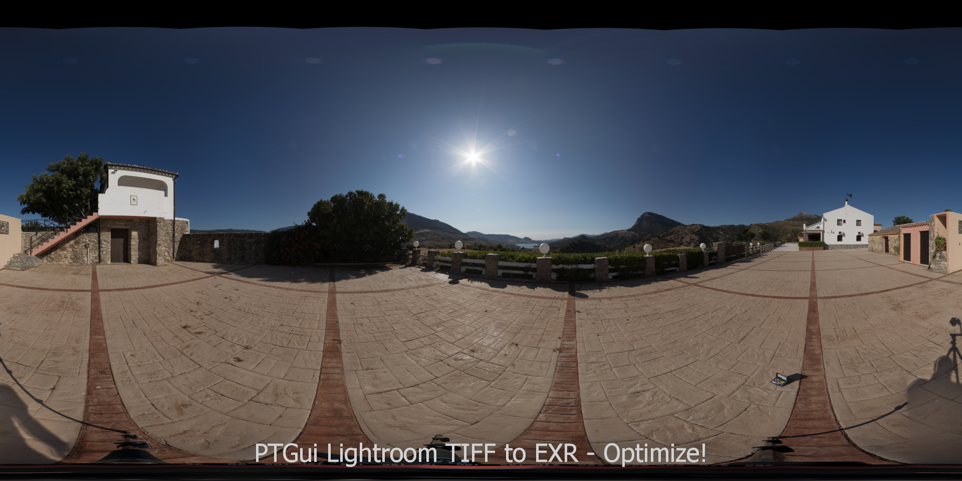
The last articles of the 2.4. series were focussing on the creation of HDRI’s mostly with DSLR cameras and exposure bracketing. A color chart (colorchecker) should be always visible in frame to make the exposure balance step later in the process easier. In my case there are a lot of image processing steps that all the image brackets have to go through: Develop the camera RAW files to TIFF and then merge and stitch all the files with PTGui Pro to an HDRI. In Nuke then comes further color balancing and exposure matching of the HDRI to a background plate or vice versa.
The goal after all the color and exposure matching steps is, that a 3D rendering result using the HDRI should fit quite well into the background plate without further tweaking.
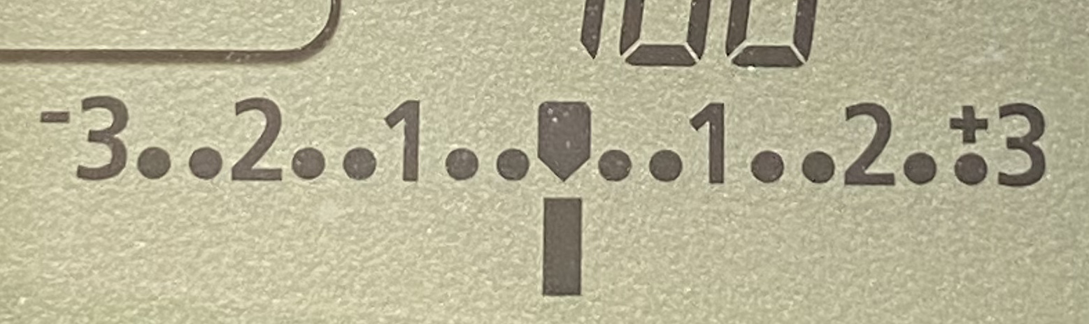
In this article I want to focus first on single exposures of my Canon 7D (MKII), starting with the “center” exposure. Later on I will continue to explore the area around the “center” exposure. Most DSLR cameras have a light meter and the center zero position stands for a “correct” exposure, whatever that means. To the left, the scale goes down to -3 stops and to the right the scale goes up to +3 stops. I did series of tests to explore how the exposure values are connected to the image output values of the sensor.
Looking at a photo has no “connection” to the exposure of the image.
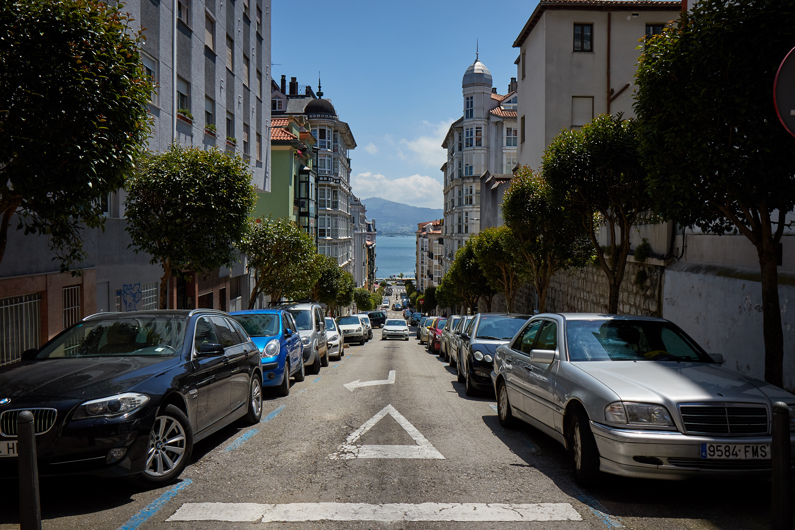
This sunny photo, taken on a holiday trip, might have been exposed “correctly” on the zero position, but a correct exposure depends on many possible camera settings. For sure, I can say that, the image result seeing here was heavily processed in Capture One and that I like the result. A “well” exposed photo is the key to get to a good looking image result.
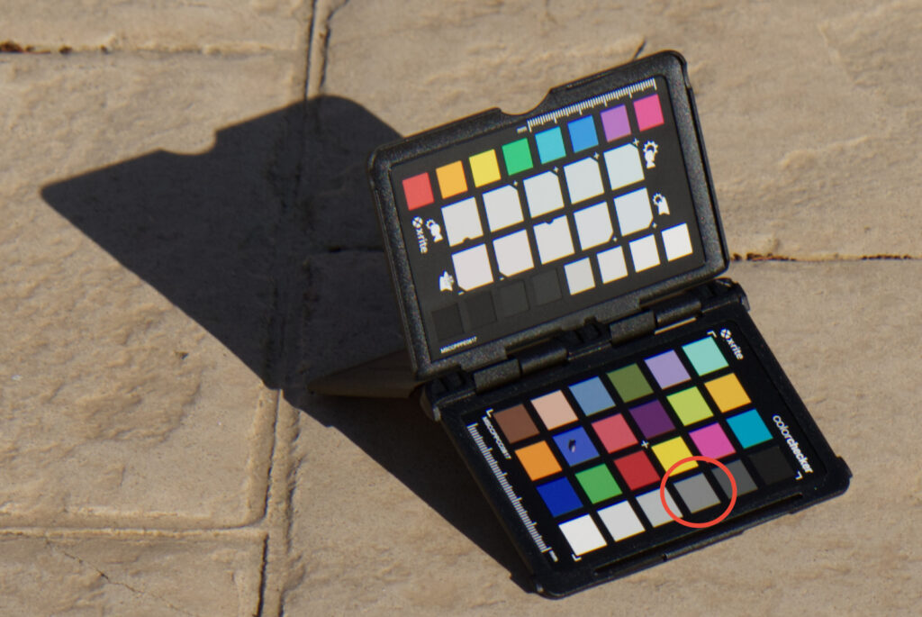
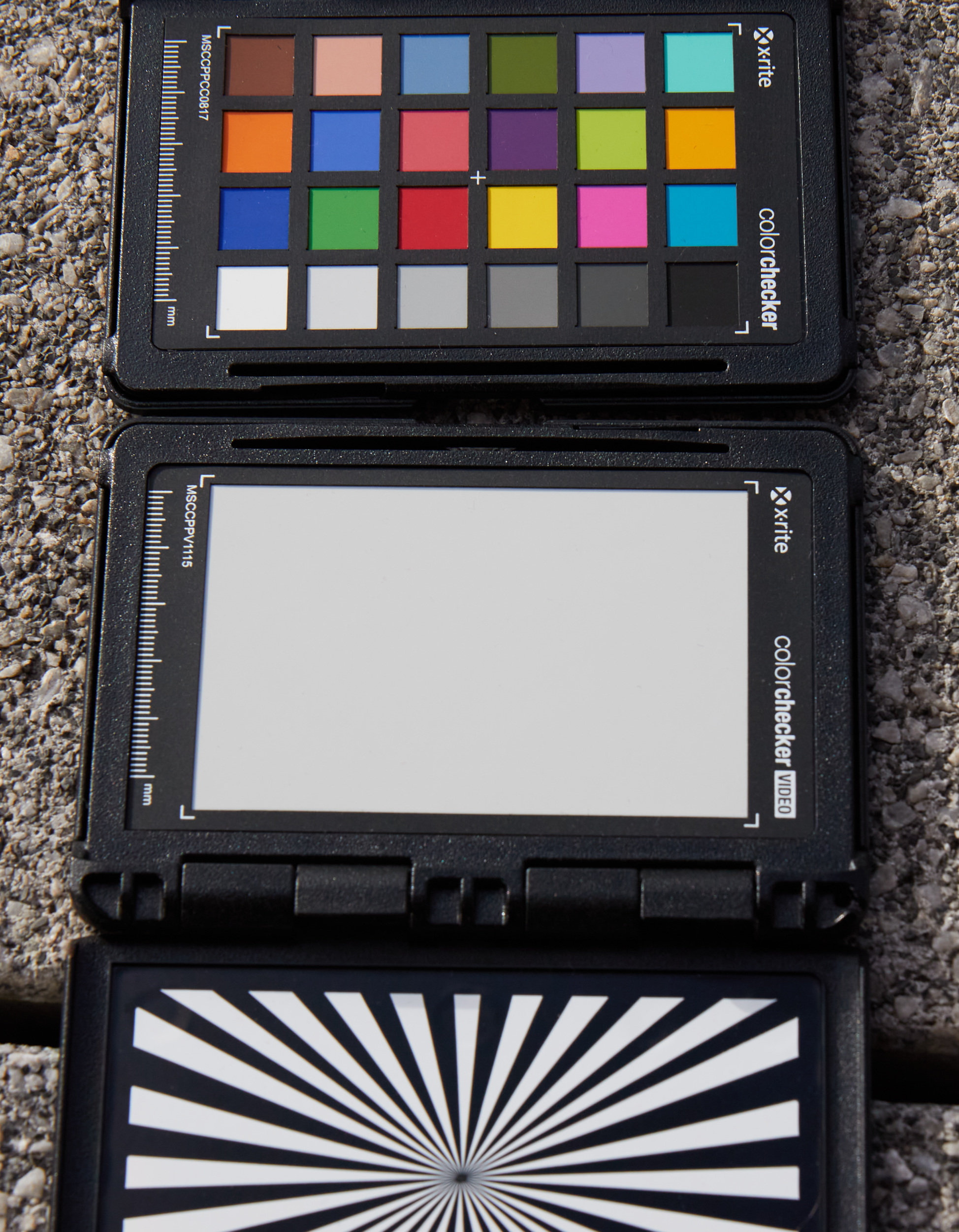
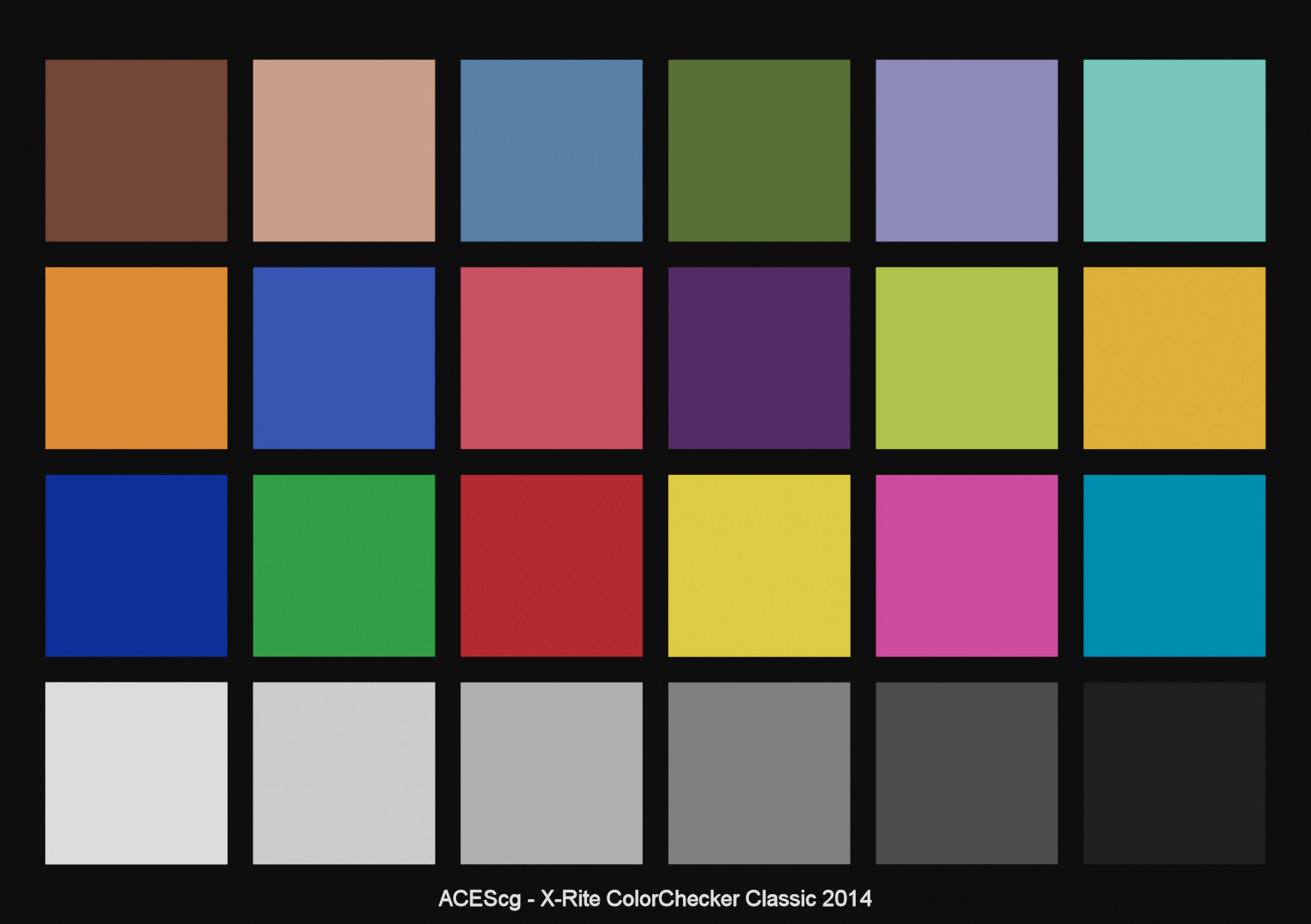
In my line of work the goal might to add convincing 3D elements into a “scene”, like I did in the last article (2.4.4. Refine and Render). To make my life easier, it is essential to know how the exposure of certain areas in an image are. A colorchecker in the frame helps to match a background plate to an HDRI for example. I need some reference in the image to be able to calibrate my exposure to. I match the exposure to the circled 18% grey patch in the photo below. Depending if I place the chart in the bright sun or in the dark shadow, the result might look very dark or way too bright. A colorchecker is not a tool to make an image pretty, but rather to check the colors and exposure, hence the name colorchecker.
Using a colorchecker for calibration
A colorchecker, visible in both the brackets for an HDRI and in a background plate serve for different purposes:
- In the image capture stage it the colorchecker is nothing more than a reference tool. I know that the 18% middle grey patch (circled) reflects roughly 18% of the incoming light.
- In the image developing stage, I can exposure balance the image to RGB 0.18 (or 18%) in scene linear. In an ACES scene-linear colorspace, the value of 0.18 has the same meaning as the 18% grey patch in the colorchecker. The image developing stage refers to the image capture stage.
That’s why the ACES colorspaces are scene-referred.
- In the output or display rendering stage, I can make sure that the middle grey patch actually reads RGB 128/128/128, or 50%, here on this website. With the help of the system tool “Digital Color Meter” on MacOS I can measure the grey value of the patch “on” this display, therefore the measurement is output- or display-referred.
Single “middle/correct” exposure
For the next example I took another a photo of a colorchecker outside in the sun. This time I photographed the big “white” reference patch (with spot metering) and set the exposure so that the indicator points to the center of the scale. In other words, the light meter indicates me a “normal” exposure.
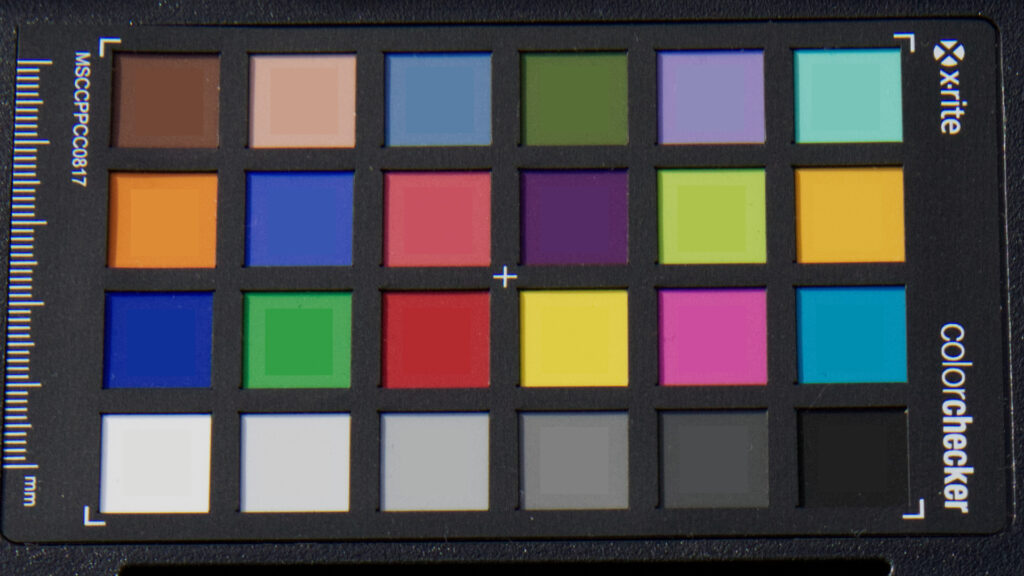
The photo was shot at ISO 100 with an aperture of f/8 and a shutter speed of 1/400. The following JPG image I “developed” in Capture One. The middle grey patch, third from the right, is adjusted or graded to read out middle grey RGB 128/128/128 in the sRGB 8-bit display referred colorspace.
This photo is now exposure and color balanced to the colorchecker for this webpage/display.
A display referred image, that is developed with Capture One or any other RAW-developer app, will end up with a luminance scale between zero and 1. Zero means “black”, or no emission from the display, and one means “white” or better to say the maximum RGB emission from the display. There are many tools available in the RAW development programs to tone map the sensor data into a nice looking result.
This photo is developed, processed, exposure and color balanced for this webpage. But the relation to the “correct” exposure of the camera was lost in the process.
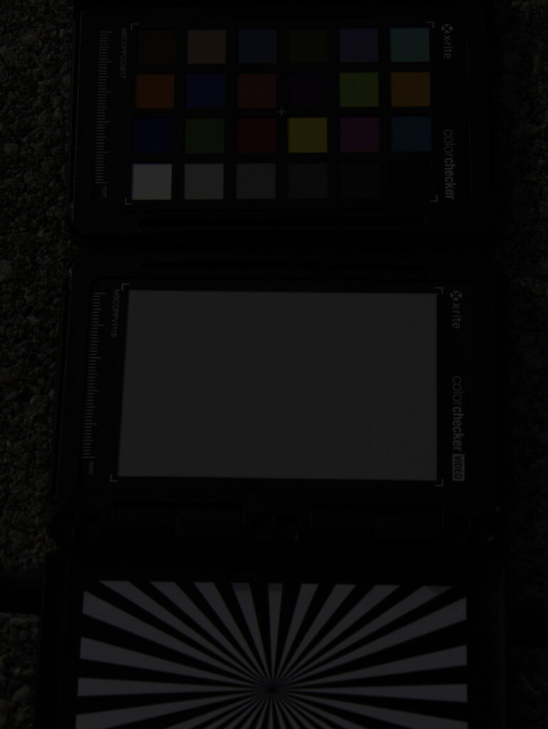
The next photo shown below is developed from the same camera raw file. This time it is converted with Affinity Photo to an EXR file (linear-sRGB). Remember: the photo was exposed to the big “white” patch in the middle of the framing. This is the “correct” exposure according to the Canon 7D MKII light meter. The scene linear value of this “white” patch reads out roughly 0.1 in Nuke. As I saved the image seen here without any view transform, the value reads on the “screen” roughly RGB 26/26/26, or in other words 10% of the possible code values between 0-255.
The image below is not exposure balanced to the colorchecker for this webpage/display. This is scene referred image data and not meant to be seen without any view transform, but here it is anyway:
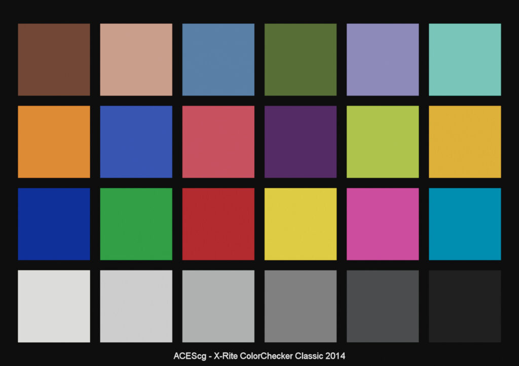
As I am still fiddling around in Nuke, I can examine the image in a scene referred colorspace and “see” how well the camera captured the 24 patches and match them to the ACEScg reference chart. To see a meaningful image, I need to turn on a view transform again. I am using the ACES (sRGB) view transform in all the tests for this article.
The EXR file coming from Affinity Photo was loaded into Nuke with the IDT “Utility-Linear-sRGB”. Then it got exposure and color balanced to the middle grey patch which is roughly at 19% in ACES, or R=0.190308 G=0.190796 B=0.189941 in ACEScg to be exact.
In the final step I overlaid the reference patches on the photographed colorchecker. And this is the result:

I can easily “correct” the processed photo to match the reference chart “better”. This was done by raising the contrast and lowering the gamma a bit, but then I am not working scene linear anymore after this correction and the 18% patch doesn’t match neither. For the next steps I will forget about the last contrast and gamma correction again to “stay” scene linear.
Seven shades of grey
For the next examples, I was taking always seven photos, or exposure brackets, instead of just one. From one photo to the next I altered the shutter speed, so that the exposure of each image is always one stop apart from the one before.
Light (photons) is received at the sensor. A bayer pattern sensor is “counting” photons from a certain low amount to a certain high amount*. In the light meter the low amount is visualized somewhere further left to the -3 stops (only sensor noise) and the high amount is visualized somewhere further right of the +3 stops. If even more photons hitting the sensor, then sensor saturation or sensor clipping will occur at some point.
I photographed a white surface with the white balance set via the
in-camera measurement and the following camera settings
(ISO 100 and f/stop 8):
| exposure | -3 | -2 | -1 | 0 | +1 | +2 | +3 |
| shutter (s) | 0.1 (1/10) | 0.2 (1/5) | 0.4 | 0.8 | 1.6 | 3.2 | 6.2 |
| scene linear | 0.013 | 0.026 | 0.050 | 0.102 | 0.208 | 0.415 | 0.835 |
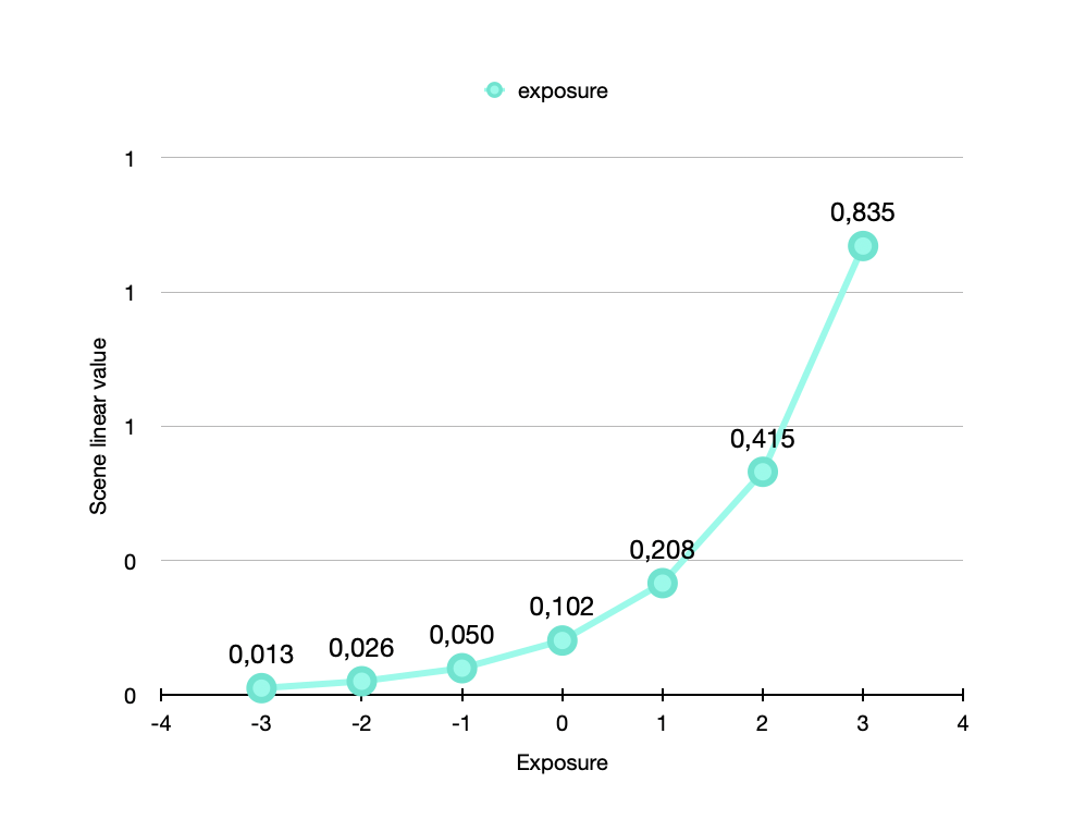
Canon places the “correct” exposure of a surface at around a scene linear value of 0.1. The image data that is coming out if the sensor and the in-camera processing has a range from zero to one.
Once I balanced the strip of images so that the center image is at around 18% (19% in ACEScg), the range of scene linear values are ranging from 0.024 to 1.543.

Three to the left and three to the right
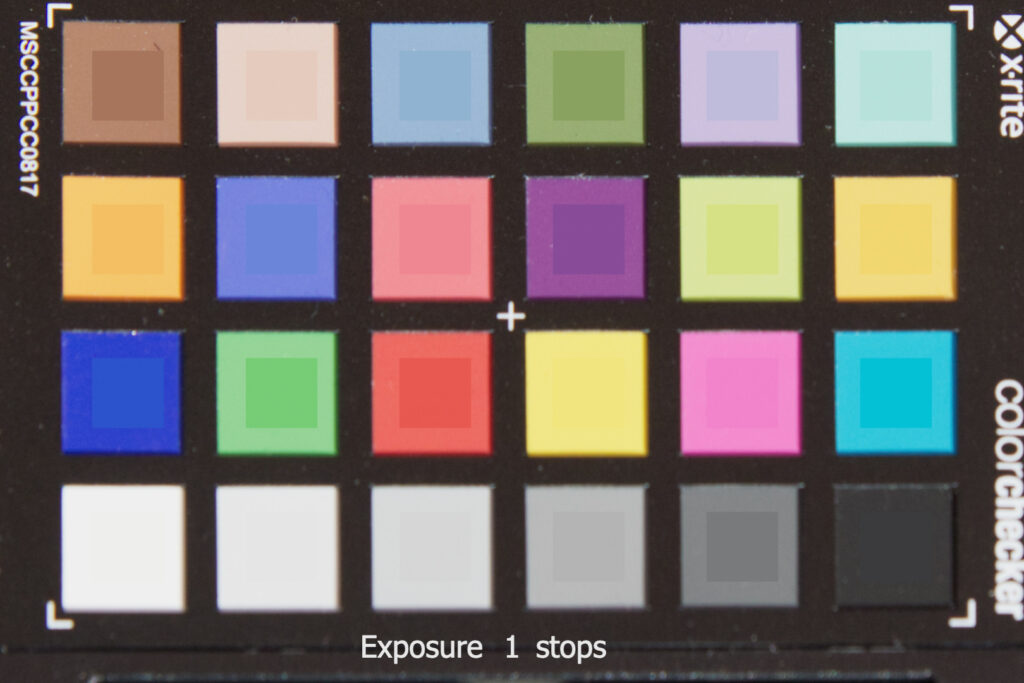
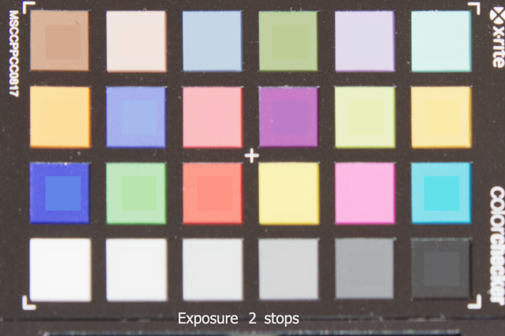
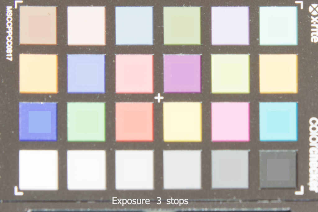
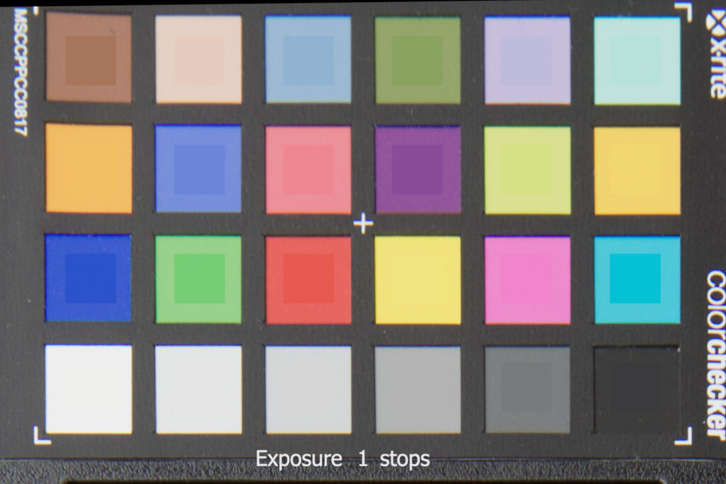
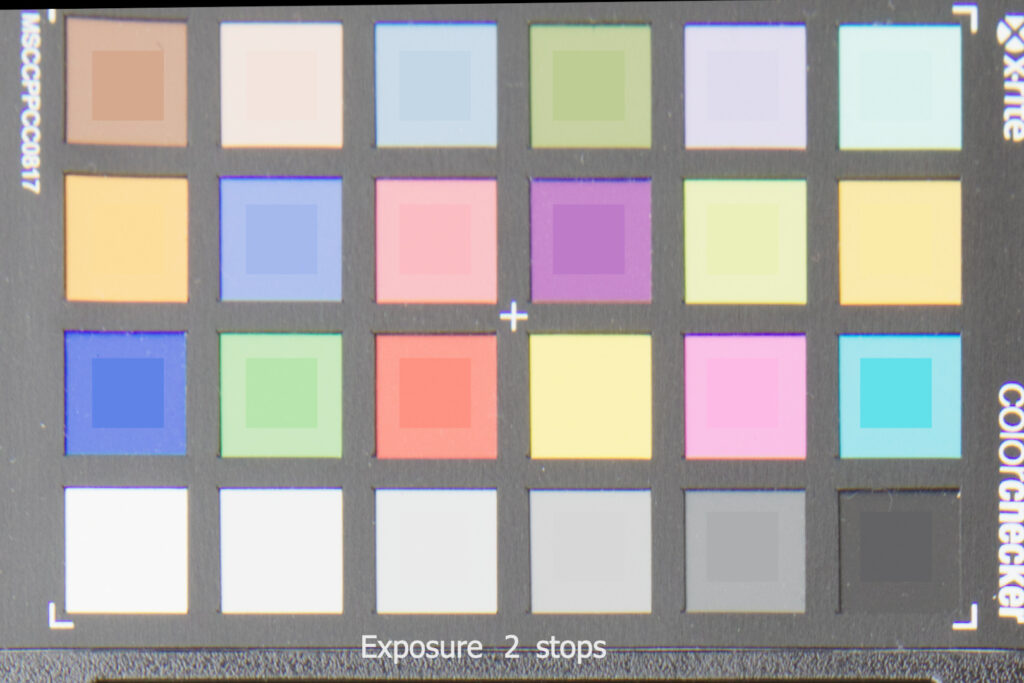
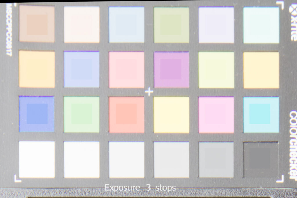
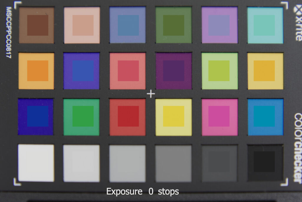
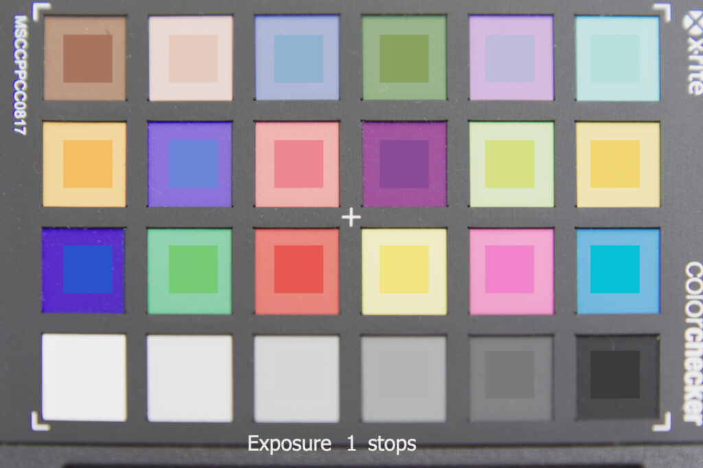
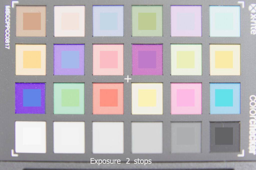
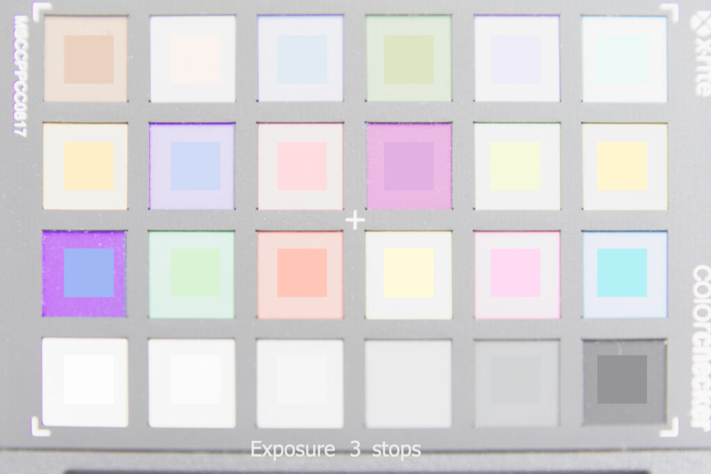
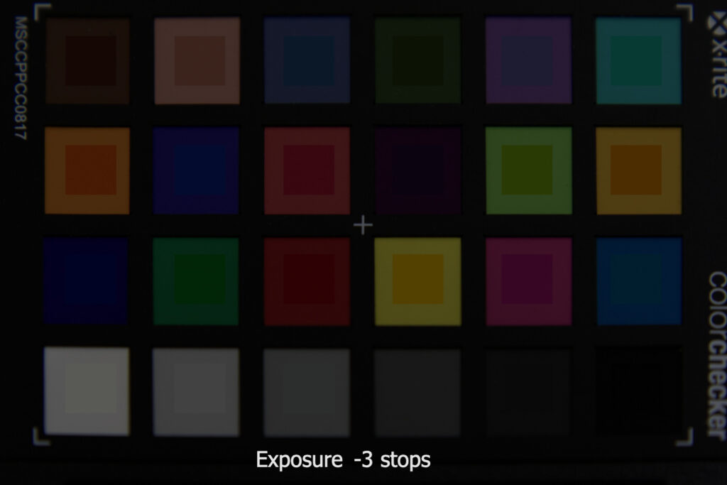
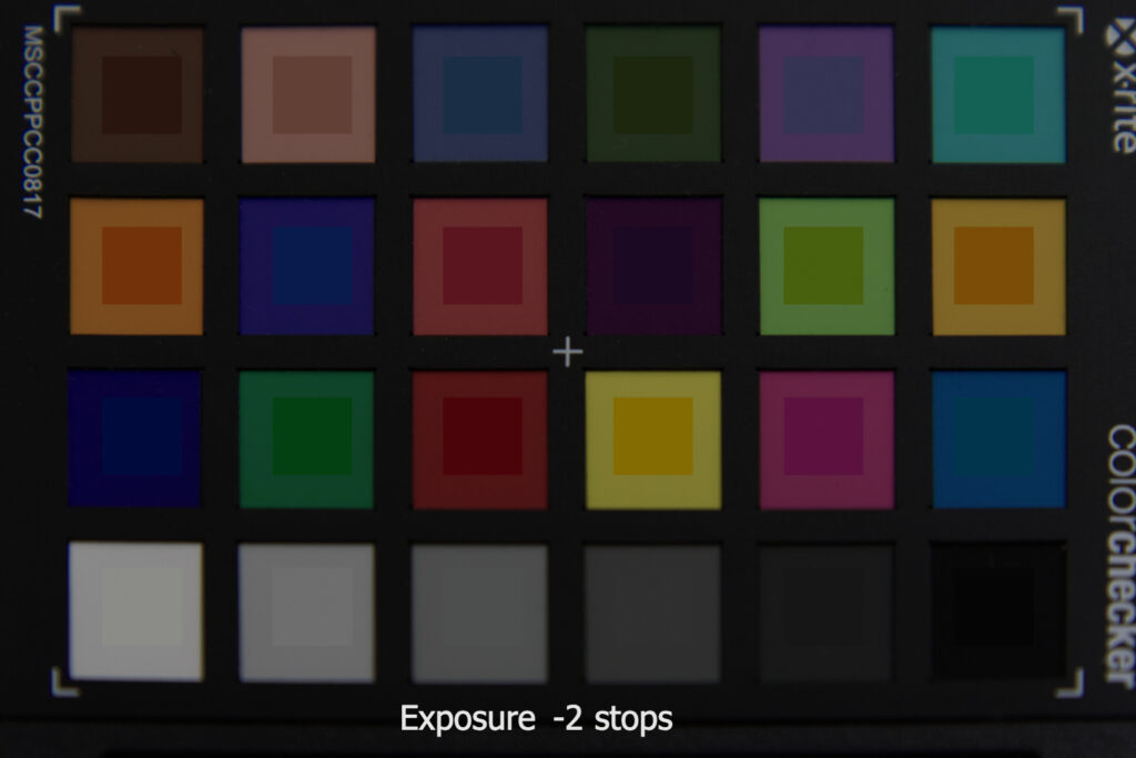
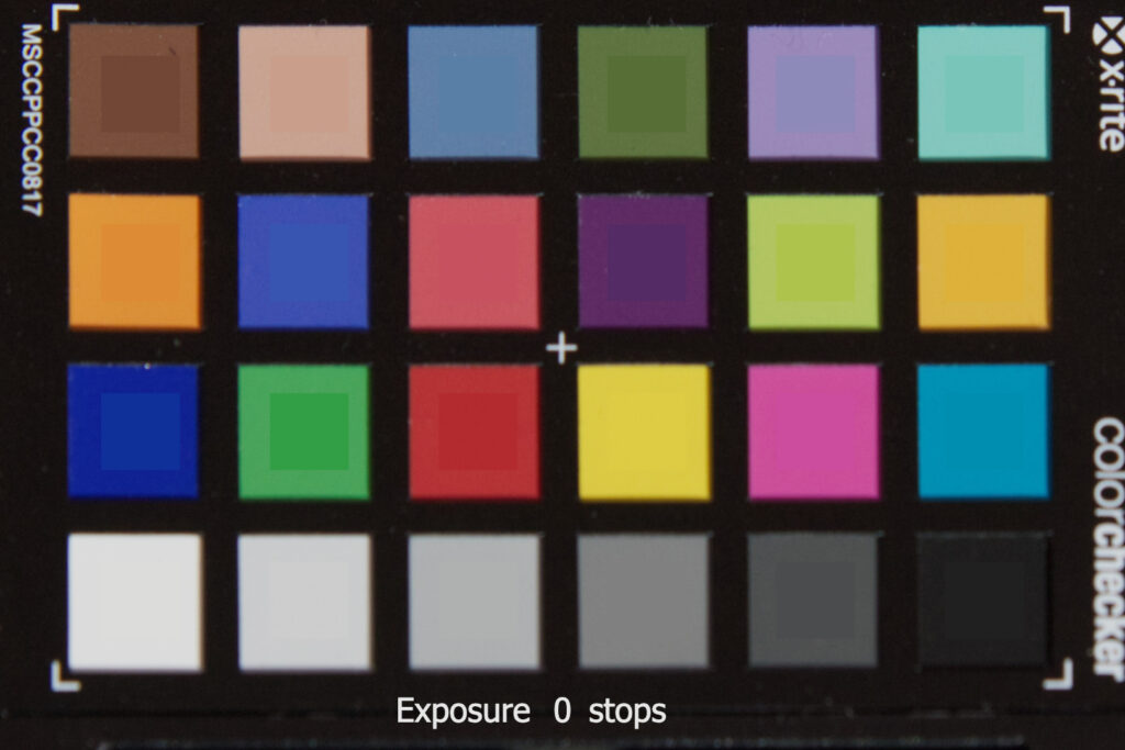
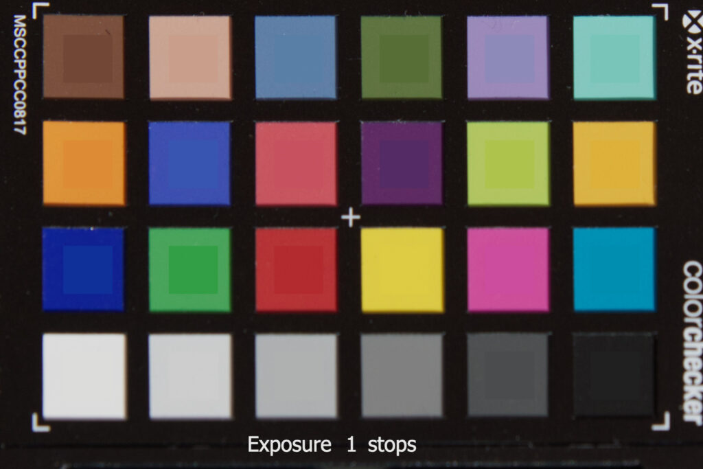
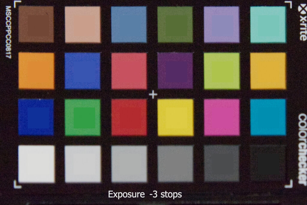
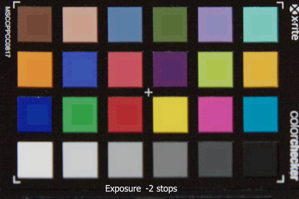
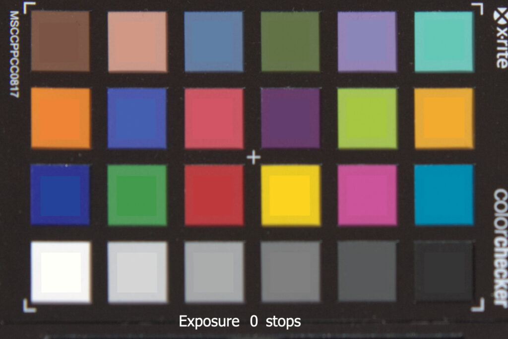
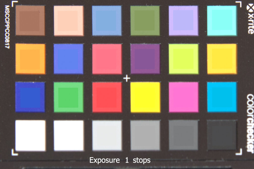
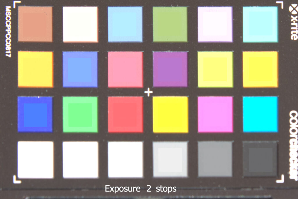
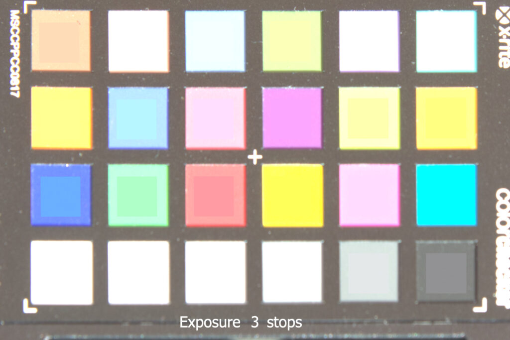
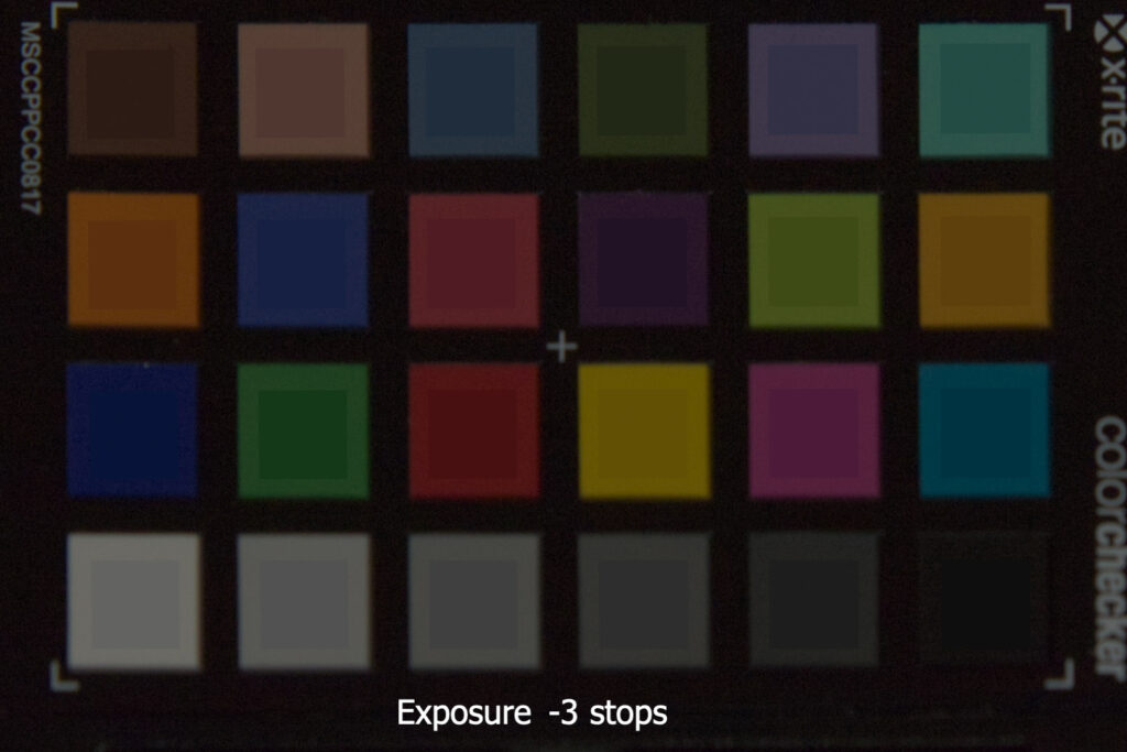
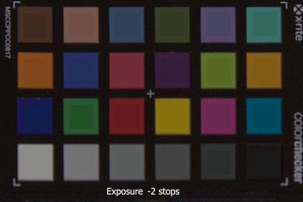
Based on the middle/correct exposure I photographed also the whole colorchecker with 7 exposures three times: (1.) outside in the sun, (2.) outside on an overcast day and (3.) inside with an indirect light mix of different LED lights from a ceiling household lamp.
The three slider-galleries start centered with the correct/middle exposure. The photographed chart is balanced to the 18% grey patch and has an additional adjustment, so that the grey patch shows RGB 128/128/128 on the screen/website. Scroll to the left lowers to lower the exposure one stop, scroll to the right to raise the exposure one stop. To the reference chart the same exposure changes are applied before the reference chart is overlaid onto the photographed colorchecker.
The first set of charts (1.) were taken on a clear sky day in the sun. The second (2.) set was taken one day later when the sky was completely overcast. The third (3.) set of images are a color-disaster. I took this set inside in a hallway which is lit only by indirect LED ceiling lamps, but they are not all the same type and have different color temperatures. This might explain why this set of exposure looks so much different than the first two.

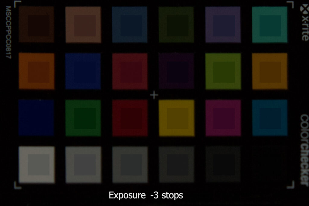
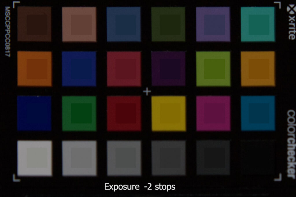
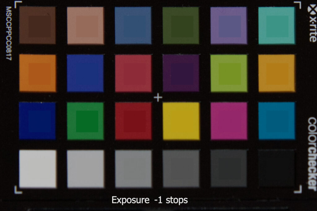
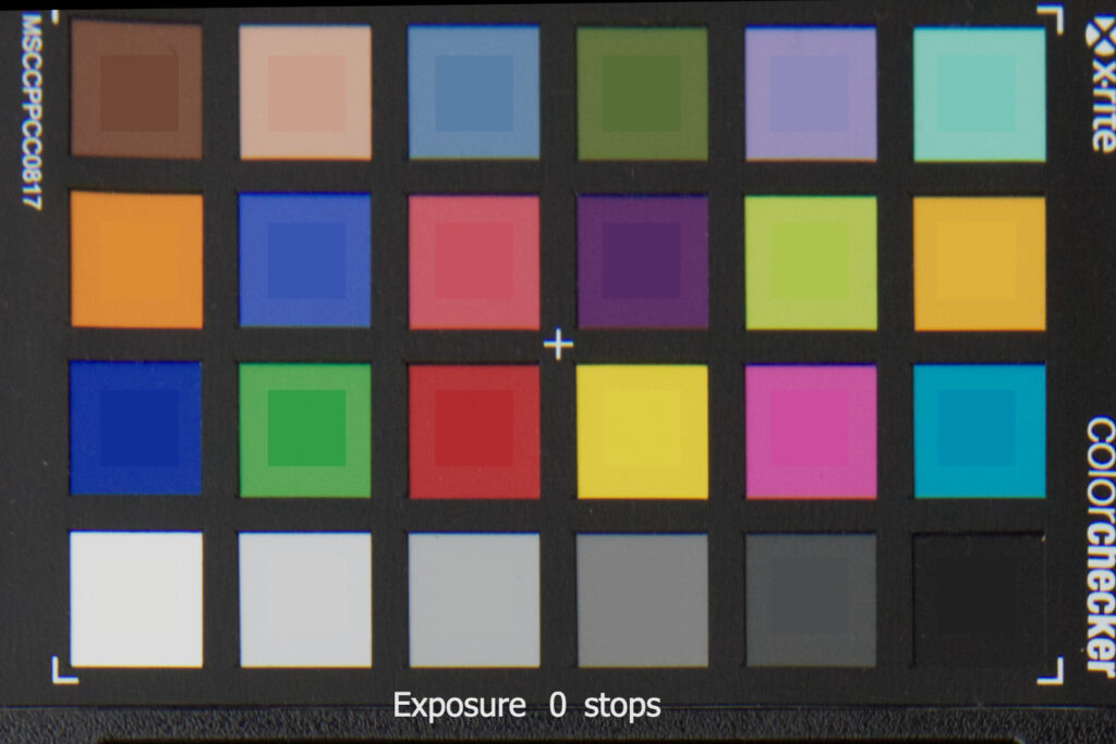
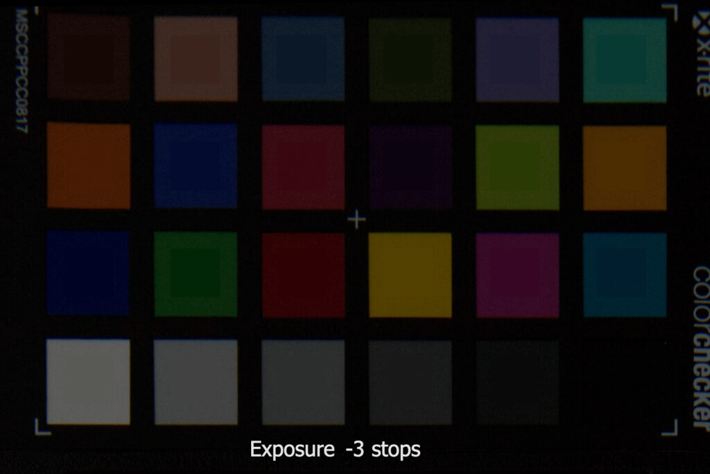
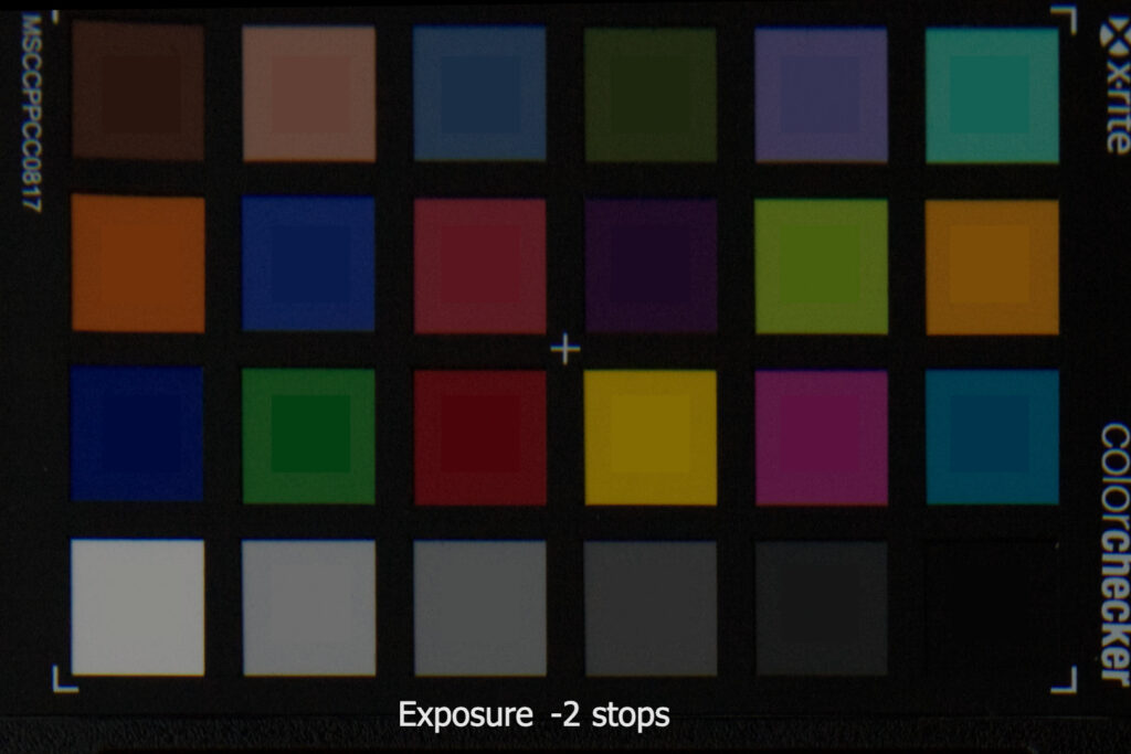
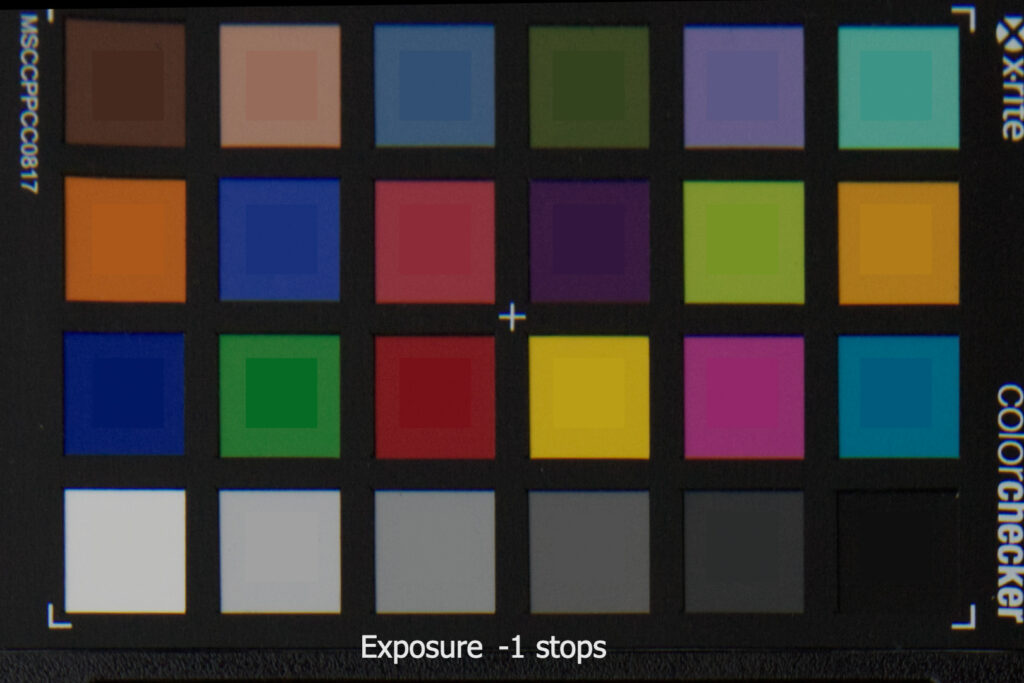
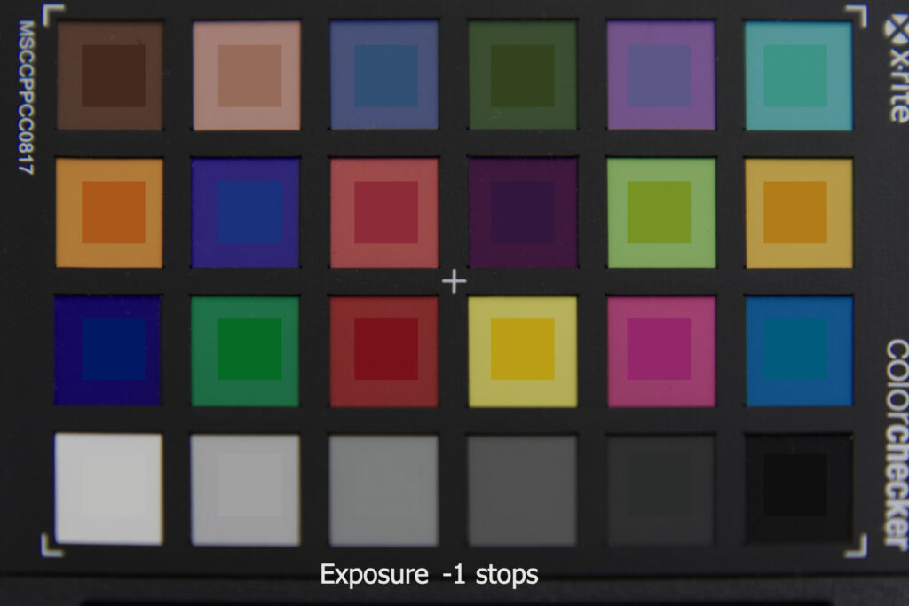
In the previous three galleries the reference chart is changing the exposure together with the photographed brackets. Another way of looking at the results is to color balance each of the seven images to the 18% grey patch and then overlay the reference color patches. The results are now keeping the same brightness, just the noise level is changing. The noise gets the most noticeable in the -3 stop exposure. In the following gallery I used the first (1.) set of photos that were taken outside in direct sunlight.

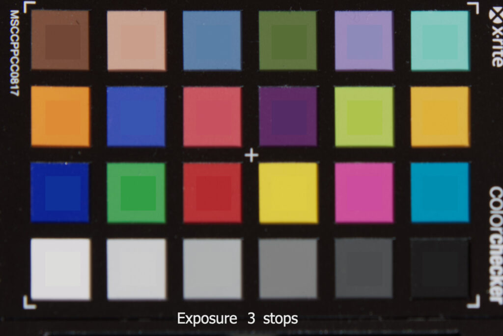

For all these tests I used the ACES color management pipeline. I know how to work in this pipeline, but I must say I don’t know what the results in the slider galleries can tell me about the whole image process. I have no idea why sometimes the lighting situation leads to results that are not matching well to the reference color patches. Also, why does the blue patch sticks out that much in the plus range, but all the other patches more in the minus range? For these questions I don’t have an answer (yet).
ACES vs. Nuke Default
Before there was a color management solution available like ACES, I was working in Nuke without color(gamut) management. To demonstrate the different results, I rendered out another (4.) set of images from Nuke-Default (non) color managed environment with the standard sRGB view transform.
Change the exposure on both image pipelines and compare the results. What are the biggest differences, which system works better?

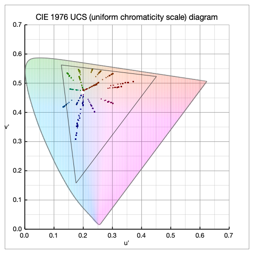
Colorchecker and gamuts
One last thing that I looked at while writing this article was the color gamut of the colorchecker. I have a small tool from the Mac AppStore called “ColorSpatioplotter“. This app reads all kinds of image files and shows that the “cyan” patch is actually out of gamut for the output Rec.709/sRGB colorspace in the working colorspace ACEScg . And the cyan patch is the only one which is out of gamut. But it is important to emphasize that the following CIE 1976 chart is showing the working colorspace ACEScg. After the display rendering stage the color patch “cyan” is inside or at the border of the sRGB/Rec.709 gamut again.
Here is the link to the reference colorchecker files, that are available from GitHub in many different colorspaces.
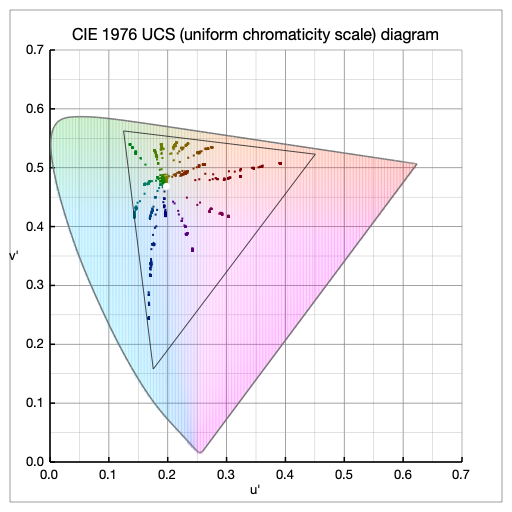
Before finishing up with this article, I also plotted all the results from the four slider galleries above. Starting with the non-ACES sRGB (4.) example first; followed by ACES sRGB direct sunlight (1.) plots; the ACES sRGB overcast sky (2.) plots; and finally the ACES sRGB inside LED light (3.) plots of the colorcheckers.
Conclusion
The biggest take away for me, after posting so many colorchecker images and tests in the whole series of posts here on this website, is: The connection between the three steps “image capture, image development and image rendering”. I always thought about these three stages as separate entities. I slowly get a better understanding of how the light meter in the camera, the resulting scene linear values after developing the image, and the view transform to “see” the image on a screen, are connected. All three steps need to be carefully considered to create a meaningful image. Only then the images might make sense on the display you are watching this webpage. The next step is look into the topic of display rendering and learn, if what I see here on a display actually makes sense to the “eye”…
* Thanks to Troy S. for this sentence and help me slowly understand what I actually “see” on a screen. For more information, head over to his blog “The Hitchhiker’s Guide to Digital Colour”.