A blurry red star on a cyan background

A while back I found this very simple example on the page Question #9 in The Hitchhiker’s Guide to Digital Colour blog from Troy Sobotka. Please the blog from the beginning, but especially Question #9 for this article.
Once in a while the blog gets updated with new topics, so I read the whole blog several times, but one image got stuck in my „head“. After numerous chats with Troy S. and a thread on ACESCentral.com, I revisited my notes of all the tests I did since I became aware of this topic. Here we go…
Note: In the ACESCentral.com thread I did comparisons including OCIO/ACES. This article will not touch anything related ACES to keep it more simple. I want to add this in another article.
I recreated the image above in Affinity Photo on a Mac in the RGB 8-Bit sRGB mode. Try it yourself in Photoshop, Pixelmator on a Mac, on iOS or on Windows PC. The result will be the same in most cases.
Pixel values have a meaning
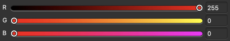
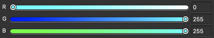
The Affinity Photo document contains a background layer filled with the RGB values 0/1/1 (in a range from zero to one) or 0/255/255, also known as cyan. The next layer on top has a star shape filled selection with the RGB values of 1/0/0 or 255/0/0 and we call it red. The second layer has a „live“ gaussian blur filter applied to blur the star and create a gradient from red to cyan.
Here is a download link to the Affinity Photo documents:
What are we looking at?
It is such a simple example, but I learned a lot from it. And I am working professionally with digital images for over 20 years.
A problem is also visible in this image. The blurry areas between the two colors are getting darker. The blurry red star has a dark halo and that does not look right.
But how should it look? How can I fix the dark halo?
The simplest way in Affinity Photo that I found is to convert the document format from 8-Bit RGB to 32-bit RGB and export another JPG (with the ICC profile embedded).

This looks better, more natural and somehow how I would expect it. There is a soft and even transition from red to cyan.
It does not matter if the image is in 8-bit mode or in 32-bit mode in Affinity Photo, the mathematical operations are the same. Something else must have changed so that the result looks better.
So what’s the difference?
The 8-bit document seems to have no display transform enabled, whereas the 32-bit document does have one.
My guess is that the 8-bit document “assumes” that the image data is already properly encoded with an inverse EOTF.
What’s an EOTF? In a display’s hardware the electronic monitor signal get converted to optical values that drive the display’s linear light output, hence the name Electro Optical Transfer Function. Before a program sends an image to the monitor a inverse EOTF should be applied to the image data. The inverse EOTF and EOTF should cancel each other out. It’s a no operation.
The 32-bit image contains floating point pixel data and needs to be “told” how it should be viewed.
The image pipeline from Affinity Photo is using the „ICC Display Transform“ on a Mac. This transform „knows“ which display is connected to the computer and adds the right inverse EOTF to the image data. The hardware in the display applies then the EOTF and the light emitting pixels in the display emit the linear light that we can see right now when you read this text and watch the images.
The 8-bit document is missing the inverse EOTF step in the image pipeline so you end up with a non-linear image data that is displayed on the screen. That non-linear ramp from red (emitting pixels) to cyan (green and blue) emitting pixels seem to create the dark halo.
In the 8-bit document I choose a “color” by setting RGB emission values in the display in a range from 0-100% (0.0-1.0) or in case of 8-bit 0-255. But I don’t set the emission values directly because I need to take into account that the image data is encoded for the display. Inside the display hardware the EOTF is always applied to the image data. Only then the data is ready to emit linear light with the help of the RGB lights in the display. The light emission can only range between 0-100%, from no light to 100% of each little RGB primary lights.
The 32-bit document contains pixel values that could mean a lot of different things, but not display emission values. Only 32-bit image data that is in a sensible range of values and has an appropriate inverse EOTF applied at the end of the image processing pipeline can drive a display in a sensible way. In other words, 32-bit EXR files need a display transform to show an image on a display.
This demonstration of the blurry red star no the cyan background is very specific. The image result looks like an ugly logo without putting my glasses on.
It is a simple demo, because there are not a lot of visual changes possible when the inverse EOTF get applied to the image data. The red and cyan sliders are set to their maximum values, therefore to the maximum light emission from the display. The transfer function leaves the minimum and maximum values untouched, but their meaning change on the way to the display.
Switching gears from Affinity Photo to Nuke
I started out digging this rabbit hole in Affinity Photo where this kind of graphic imagery is found more often than in Nuke. Nuke started from the beginning as a tool that always separated the image pipeline in the working space (linear by default) and a view transform. In the default Nuke settings the view transform is called sRGB. This is more or less the inverse EOTF that a typical sRGB display expects.
Please check this video from FilmLight about another rabbit hole: “sRGB… We Need To Talk” (45 min.)
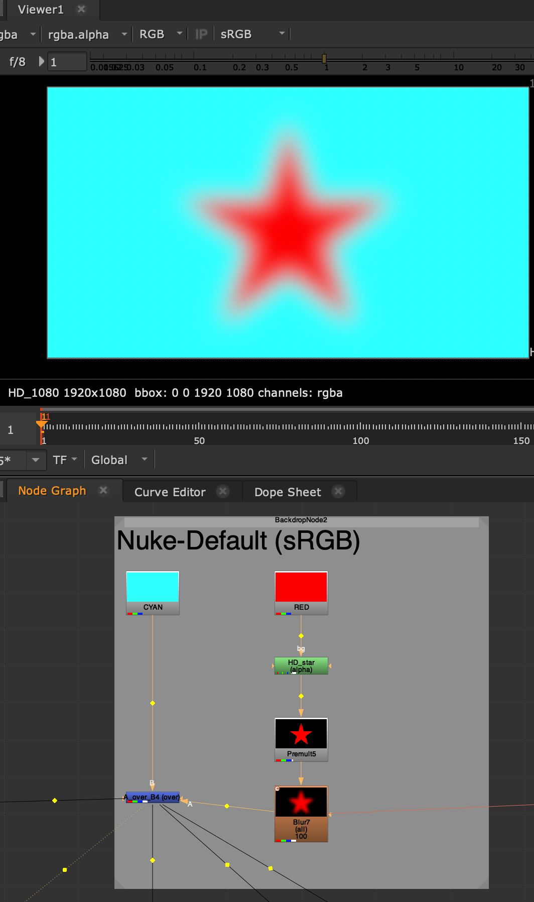
The image looks right from the start.
The script in the node graph is essentially doing the same operations that are happening in Affinity Photo. Both programs calculate their operations in the same way, but use different buffers that can hold more or less numbers.
Let’s turn of the view transform to “NONE” and thereby not adding the inverse EOTF in the image pipeline. The result looks now again the same as in Affinity Photo with the 8-bit document.
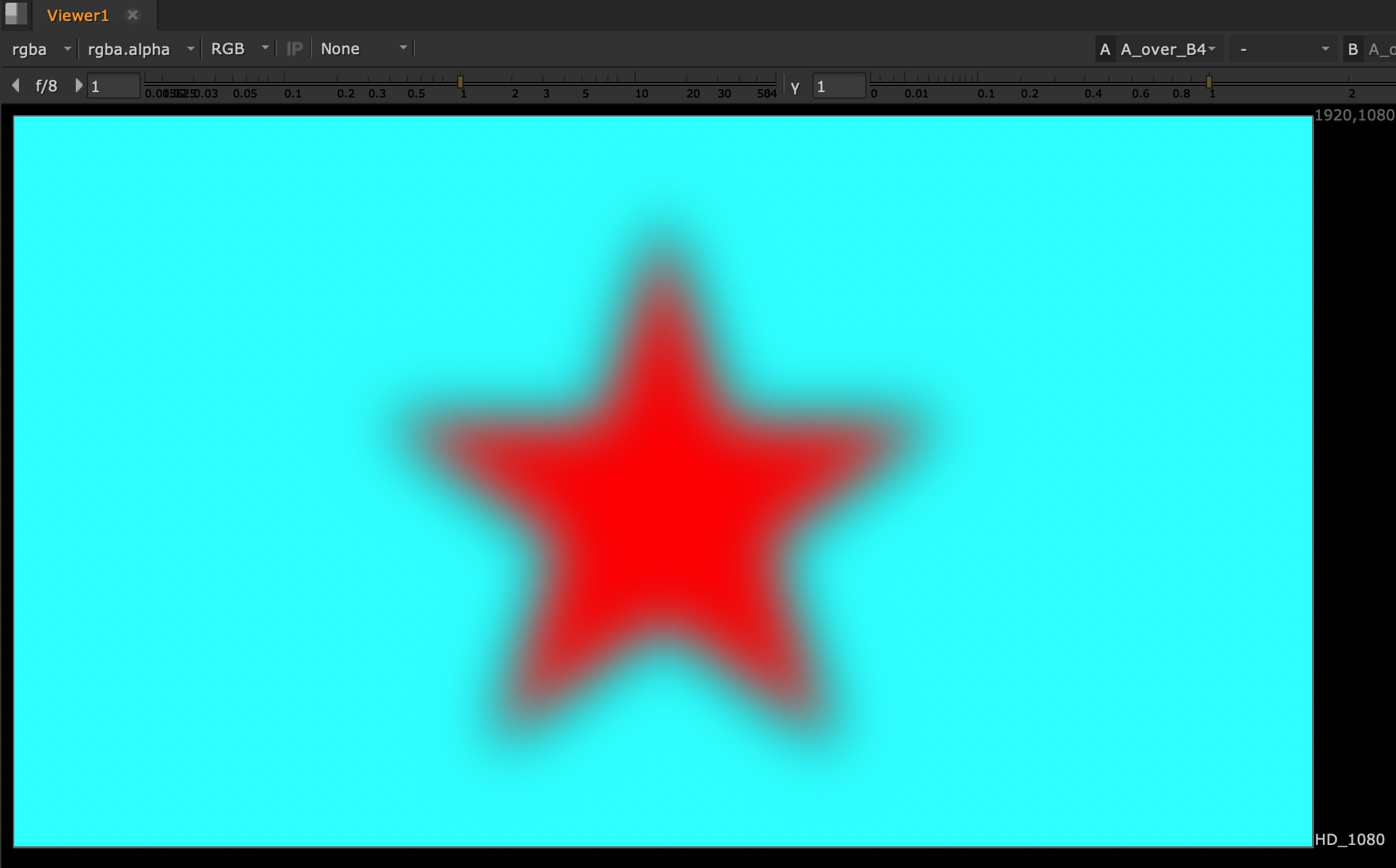
This means adding the inverse EOTF is a crucial step to get a sensible image from the display to your eyes. The transition area between full red emission to full green and blue (and no red) emission has to be linear and with values between zero and one, otherwise the image will look unnatural.
So let’s turn the sRGB view transform on again add a grade node in the node tree to alter the image result.
But of course always before the inverse EOTF gets applied.
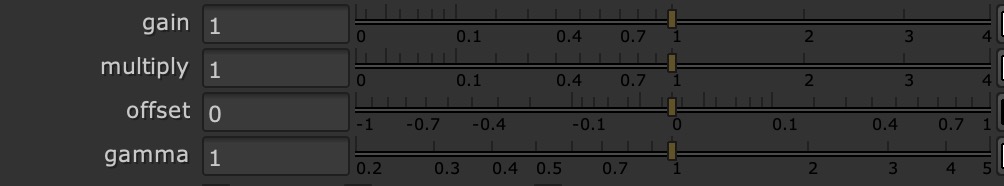
Nuke processing pipeline is very simple and clever. In the next video I will only use gain, offset and gamma to make changes to the image result.
When you hover with the mouse pointer over a number field, a description of the internal variable name appears. As you will see in a moment it makes sense that gain is labeled “white” and offset is called “add”.
Also note that the numbering scale in the grade node is different from programs like Affinity Photo. These are not linear but logarithmic scales.
First I will only use gain (white) and offset (add) to change the image. You will see that the numbers on the log scale are actually matching the direct light emission values (in percent) of my display.
Enter 0.5 for gain in the range between 0.0-1.0 and the slider will end up a bit higher than around 2/3 of the way, 0.73 or 73% emission to be exact.

In Question #21 of the “The Hitchhiker’s Guide to Digital Colour” I learned more about the math used in this transfer function.
The gain and offset sliders control directly the levels of light emission from the display. I was never aware of that fact. This works only with sRGB displays and the specific inverse EOTF.
What is happening here?
As I described already, the emission of red and cyan (green & blue display elements) is already set to the maximum before I change any value in the grade node.
White=1.00, that is display white, more is not possible. I cannot emit more light than 100%. The first part of the animation lowers white till zero or 0%. The image appears black, there is no emission from the display. Then the slider moves back to the initial value of 1.00.
Next Add=0.00, no additional light emission is added to all three RGB channels. The animation changes until Add=1.00 or 100%. The image appears white, the maximum that the display can emit light. On the way you can see a white halo around the star. The gradient contains pixel values where red has additional green and blue emission and cyan which was already some red emission mixed in. The areas in the gradient will read 1.0 or 100% earlier than the pure red and cyan pixels.
These two operations are the only ones I can be expressed on the display: Gain from 1-0 and Offset from 0-1.
The next parts of the animation will show more funky results. Raising the gain over 1.0 or 100%, moving the offset slider into negative values. Both parts will look broken.
Lastly the gamma value gets animated which result in a black or white halo. So to keep the image intact, I should leave it at 1.00.
How to continue?
There will be a second article looking into other EOTF’s as well as OCIO/ACES. The topic gets quickly more complicated as soon as I try to touch WideGamut displays.